Landform Classification

Classifies a landscape into slope-position or landform classes on the basis of the Topographic Position Index (TPI; see tpi) and slope, following Weiss (2001) and Jenness (2006). Two classifications are available: the six-class Slope Position Classification, based on one TPI scale, and the ten-class Landform Classification, based on a small and a large TPI scale.

Usage

landform(
  x,
  scale = 3,
  sn = 3,
  ln = 7,
  class.type = c("slope.position", "landform.classification"),
  descriptive = FALSE,
  leg.pos = NULL,
  leg.cex = 0.8,
  units = c("cells", "map"),
  shape = c("square", "circle", "annulus"),
  inner = NULL,
  centre = FALSE,
  std = c("global", "local"),
  tpi.thr = c(0.5, 1),
  lf.thr = 1,
  slope.thr = 5,
  plot = TRUE,
  shade = c("none", "slope", "hill"),
  col = NULL
)

Arguments

x: A single-layer SpatRaster (or a RasterLayer, which is converted internally) representing elevation. A projected coordinate system with the same horizontal and vertical units (e.g. metres) is recommended, since slope (and hence the slope threshold) depends on it.
scale: Neighbourhood size for the Slope Position Classification. With units = "cells" (default), the width of the moving window in cells (odd integer >= 3); with units = "map", the radius (half-width for square windows) in map units (metres for longitude/latitude rasters). Default 3.
sn, ln: Small and large neighbourhood sizes for the Landform Classification, in the same units as scale. Defaults 3 and 7; ln must be larger than sn.
class.type: Either "slope.position" (default) or "landform.classification".
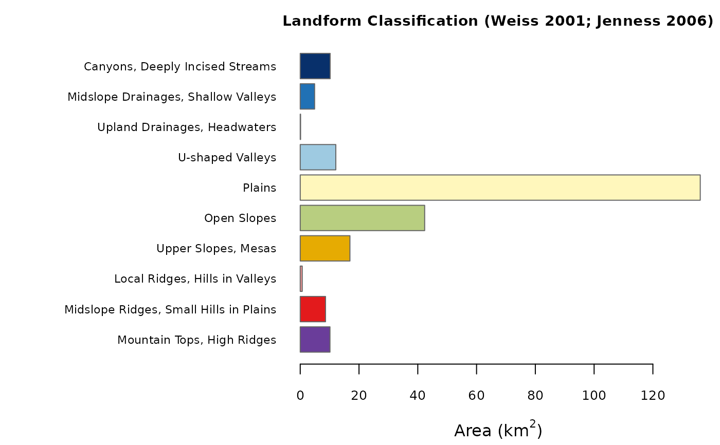
descriptive: Logical. If TRUE, a bar plot of the area of each class is drawn in addition to the map (default FALSE). The descriptive statistics are always computed and stored in the returned object (see Value).
leg.pos: Position of the legend of the map, as a keyword accepted by legend (e.g. "topright"). The default, NULL, places the legend outside the map, to its right, so that no data are hidden.
leg.cex: Magnification of the legend text. Default 0.8.
units: Either "cells" (default) or "map"; see scale.
shape: Neighbourhood shape: "square" (default), "circle", or "annulus". See tpi.
inner: Inner radius (or radii) of the annulus, in the same units as scale: one value for the Slope Position Classification, two values (for sn and ln) for the Landform Classification. Ignored unless shape = "annulus".
centre: Logical. Include the focal cell in the neighbourhood mean? Default FALSE. See tpi.
std: TPI standardisation: "global" (default; Weiss 2001, Jenness 2006) or "local" (as in landform <= 0.2). See tpi for the difference, which can be substantial.
tpi.thr: Two increasing positive thresholds (in standard deviation units) used by the Slope Position Classification. Default c(0.5, 1) (Weiss 2001).
lf.thr: Threshold (in standard deviation units) separating low, mid and high TPI in the Landform Classification. Default 1 (Weiss 2001).
slope.thr: Slope threshold, in degrees, separating flat from sloping terrain. Default 5 (Weiss 2001).
plot: Logical. Draw the map of the classes? Default TRUE.
shade: Relief shading drawn underneath the classes: "none" (default), "slope" (slopeshade) or "hill" (hillshade). See plot.landform.
col: Optional vector of colours, one per class. By default the Slope Position Classification uses an ordinal blue-to-brown palette (valley to ridge) that remains readable with the common forms of colour blindness; the Landform Classification groups hues by landform family (drainages and valleys in blues, plains and slopes in yellows and greens, ridges and tops in oranges, reds and purple). With ten classes no palette is fully colour-blind safe; supply your own if needed.

Value

An object of class "landform": a list with elements

classes: a categorical SpatRaster of the classes (integer codes with class names as levels and a colour table); per-class layers can be obtained with class_layers;
tpi: a SpatRaster with the raw (elevation units) and standardised TPI layers used in the classification;
slope: a SpatRaster of slope (degrees);
stats: a data frame with, for every class, the number of cells, the area (km\(^2\)), the percentage of the classified area, and the mean elevation and slope;
dem: the input elevation raster;
params: a list of the settings used.

The object has print, summary and plot methods (see plot.landform). The map (and, with descriptive = TRUE, the bar plot of class areas) is drawn as a side effect when plot = TRUE; the object is returned invisibly in that case.

Details

Slope Position Classification (Weiss 2001). With \(z\) the standardised TPI, \(t_1 < t_2\) the values of tpi.thr, and \(s\) the slope in degrees:

1 Valley	\(z \le -t_2\)
2 Lower Slope	\(-t_2 < z \le -t_1\)
3 Flat Slope	\(-t_1 < z < t_1\) and \(s \le\) `slope.thr`
4 Middle Slope	\(-t_1 < z < t_1\) and \(s >\) `slope.thr`
5 Upper Slope	\(t_1 \le z \le t_2\)
6 Ridge	\(z > t_2\)

Landform Classification (Weiss 2001; Jenness 2006). With \(SN\) and \(LN\) the standardised TPI at the small and large scales, and \(t\) the value of lf.thr:

1 Canyons, Deeply Incised Streams	\(SN \le -t\), \(LN \le -t\)
2 Midslope Drainages, Shallow Valleys	\(SN \le -t\), \(-t < LN < t\)
3 Upland Drainages, Headwaters	\(SN \le -t\), \(LN \ge t\)
4 U-shaped Valleys	\(-t < SN < t\), \(LN \le -t\)
5 Plains	\(-t < SN < t\), \(-t < LN < t\), \(s \le\) `slope.thr`
6 Open Slopes	\(-t < SN < t\), \(-t < LN < t\), \(s >\) `slope.thr`
7 Upper Slopes, Mesas	\(-t < SN < t\), \(LN \ge t\)
8 Local Ridges, Hills in Valleys	\(SN \ge t\), \(LN \le -t\)
9 Midslope Ridges, Small Hills in Plains	\(SN \ge t\), \(-t < LN < t\)
10 Mountain Tops, High Ridges	\(SN \ge t\), \(LN \ge t\)

Both sets of rules assign every cell to exactly one class.

Edges and NA cells. Slope cannot be computed for the outermost cells of the raster and for cells adjacent to NA cells; these cells are left unclassified (NA) for every class, so that the class frequencies are not biased by edge effects.

Area. Class areas are computed with cellSize, and are therefore correct also for longitude/latitude rasters; for projected rasters they are ground areas, which may differ slightly from the nominal cell area (resolution squared) because of the scale distortion of the projection. If the raster has no coordinate reference system, map units are assumed to be metres.

Reproducing results of landform <= 0.2. Use std = "local", centre = TRUE (with the default square window in cells). Cells whose standardised TPI equalled exactly \(t_1\) were left unclassified by earlier versions and are now classified as Upper Slope; edge cells are now consistently NA.

References

Jenness, J. (2006). Topographic Position Index (tpi_jen.avx) extension for ArcView 3.x, v. 1.2. Jenness Enterprises.

Weiss, A. (2001). Topographic Position and Landforms Analysis. Poster presentation, ESRI User Conference, San Diego, CA.

See tpi for references on the TPI and its standardisation.

Examples

dem <- malta_dtm()

# Slope Position Classification, 9 x 9 cell window
sp <- landform(dem, scale = 9)

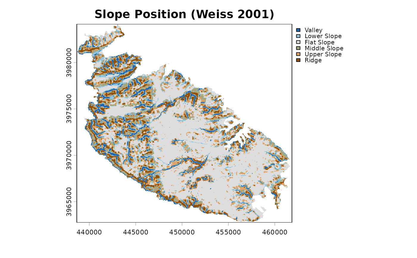sp
#> <landform> Slope Position Classification (Weiss 2001) 
#>   neighbourhood : scale = 9 in cells (window width) - square (focal cell excluded) 
#>   TPI standard. : global 
#>   classified    : 151209 cells, 242.108 km2
#> 
#>  code        class area_km2 percent
#>     1       Valley   18.525     7.7
#>     2  Lower Slope   20.158     8.3
#>     3   Flat Slope  117.906    48.7
#>     4 Middle Slope   32.303    13.3
#>     5  Upper Slope   29.647    12.2
#>     6        Ridge   23.569     9.7
summary(sp)
#>   code        class cells  area_km2   percent mean_elev mean_slope
#> 1    1       Valley 11570  18.52517  7.651614  69.89451   9.338478
#> 2    2  Lower Slope 12590  20.15838  8.326192  71.80379   6.280658
#> 3    3   Flat Slope 73638 117.90586 48.699686  74.13968   2.352399
#> 4    4 Middle Slope 20175  32.30305 13.342410  86.22553   8.891103
#> 5    5  Upper Slope 18516  29.64684 12.245291  94.85939   5.342676
#> 6    6        Ridge 14720  23.56875  9.734807 110.86959   7.932017

# Landform Classification, circular neighbourhoods of 120 m and 480 m
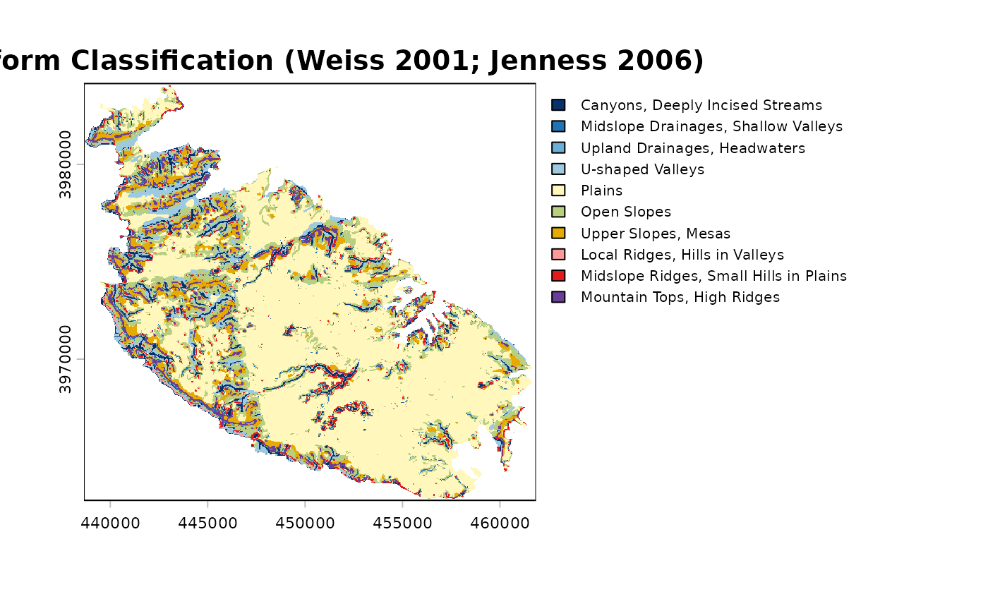
lf <- landform(dem, class.type = "landform.classification",
               sn = 120, ln = 480, units = "map", shape = "circle")


# \donttest{
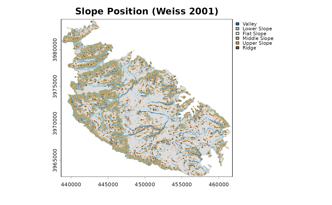
# the standardisation used by landform <= 0.2, for comparison
sp_local <- landform(dem, scale = 9, std = "local", centre = TRUE)

# }

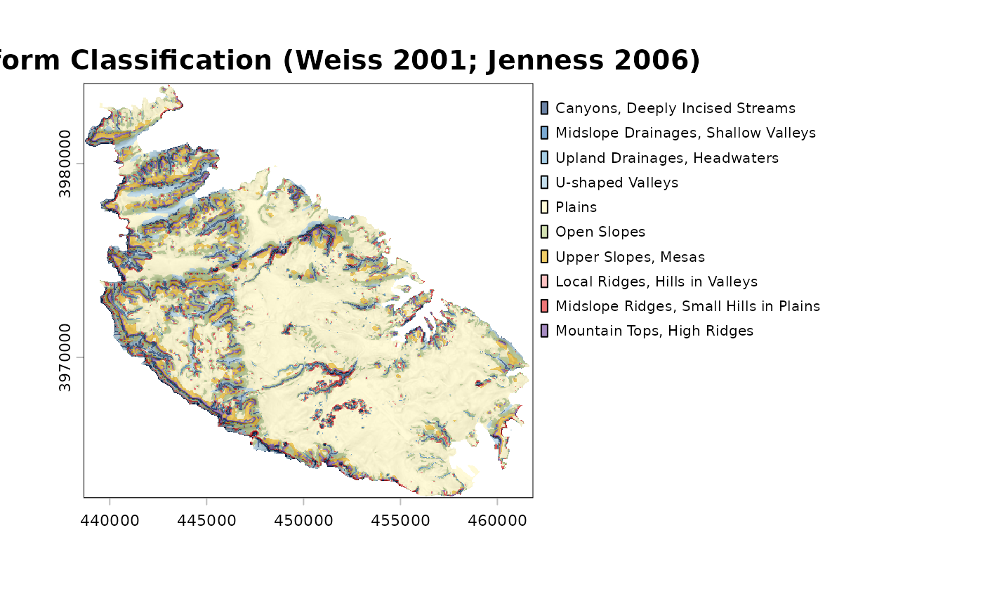
# the same, over a slopeshade, with the bar plot of class areas
plot(lf, shade = "slope")

plot(lf, what = "area")


# one layer per class
layers <- class_layers(lf)